Contents
- Linear operation
- Inverting amplifier example
- Limit on input for 12-V supply
- Limit on input for 20 mA out of op amp
- Saturation Conditions
- An example of saturation with two signals
- Summing Junction with two signals
- Non-Ideal Op Amps: Finite Gain
- Lorentzian Spectrum to be used for gain-bandwidth analysis
- Non--Ideal Op Amp: Gain and Bandwidth
%%% opamp.m  Notes for Op Amp lectures
%
% by Chuck DiMarzio
%    Northeastern University
%    September 2009
%
% Run at
moose=clock;
runtime=[date,' at ',sprintf('%2.0f',moose(4)),':',sprintf('%02.0f',moose(5))]
%
runtime =
14-Sep-2009 at 10:57
Linear operation

No current into or out of input terminals
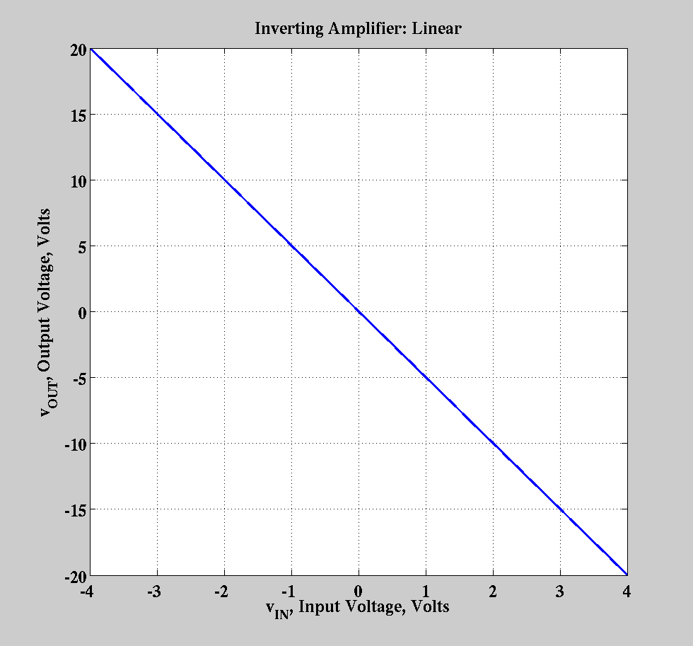
Inverting amplifier example

R_1=1000;R_2=5000;R_L=500;
A_v = -R_2/R_1  % Voltage gain
A_vdB=20*log10(abs(A_v))
A_i=A_v^2*R_1/R_L  % Current Gain
A_idB=20*log10(abs(A_i))
A_p=A_v*A_i
A_pdB=10*log10(abs(A_p))
%

v_INdemo=[-4:0.1:4];
v_OUTdemo=v_INdemo*A_v;
fig1=figure;plot(v_INdemo,v_OUTdemo);
grid on;
xlabel('v_{IN}, Input Voltage, Volts');
ylabel('v_{OUT}, Output Voltage, Volts');
title('Inverting Amplifier: Linear');
A_v =
    -5
A_vdB =
   13.9794
A_i =
    50
A_idB =
   33.9794
A_p =
  -250
A_pdB =
   23.9794
Limit on input for 12-V supply
disp('Limit on input for 12-V supply ');
v_OUTvlimit=[-12,12]  % Range of Voltages
v_INvlimit=v_OUTvlimit./A_v^2*R_1/R_L
Limit on input for 12-V supply
v_OUTvlimit =
   -12    12
v_INvlimit =
   -0.9600    0.9600
Limit on input for 20 mA out of op amp
disp('Limit on input for 20 mA out of op amp');
i0=20e-3*[-1,1] % Output current in Amps
r_par=1/(1/R_2+1/R_L)
v_OUT=i0*r_par  % Voltage out at these currents
v_INilimit=v_OUT./A_v      % Voltage in
Limit on input for 20 mA out of op amp
i0 =
   -0.0200    0.0200
r_par =
  454.5455
v_OUT =
   -9.0909    9.0909
v_INilimit =
    1.8182   -1.8182
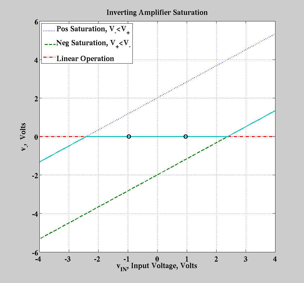
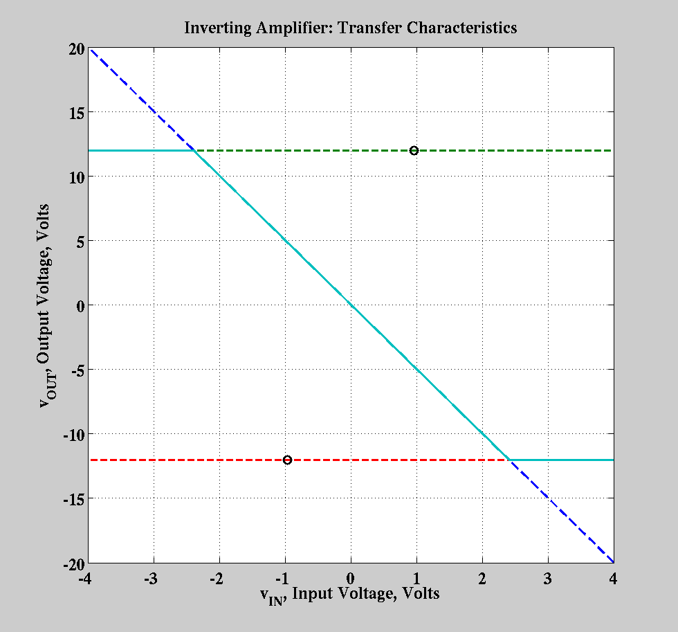
Saturation Conditions
Increase R_3 or use a different op amp so that the current limit
discussed above does not occur.
v_OUTp=v_OUTvlimit(2);  % Output saturated to positive power supply rail
v_OUTn=v_OUTvlimit(1);  % Output saturated to negative power supply rail
% First plot the voltage at the inverting input as a piecewise linear
% plot.  First three lines show the individual pieces, and the last line
% puts them together.  The dots show the boundaries.
%
v_minusp=v_INdemo+R_1/(R_2+R_1)*(v_OUTp-v_INdemo);  % Voltage divider
v_minusn=v_INdemo+R_1/(R_2+R_1)*(v_OUTn-v_INdemo);  % Voltage divider
fig2=figure;plot(v_INdemo,v_minusp,':',v_INdemo,v_minusn,'--',...
                 v_INdemo,zeros(size(v_INdemo)),'-.',...
                 v_INdemo,max(v_minusn,min(0,v_minusp)),'-',...
                 v_INvlimit,zeros(size(v_INvlimit)),'ko');
grid on;
xlabel('v_{IN}, Input Voltage, Volts');
ylabel('v_{-},  Volts');
title('Inverting Amplifier Saturation');
legend('Pos Saturation, V_-<V_+',...
       'Neg Saturation, V_+<V_-',...
       'Linear Operation','Location','NorthWest');

% Now plot the output voltage as a piecewise linear
% plot.  First three lines show the individual pieces, and the last line
% puts them together.  The dots show the boundaries.
%
v_OUTwithsat=min(max(v_OUTdemo,-12),12);
fig3=figure;plot(v_INdemo,v_OUTdemo,'--',...
                 v_INdemo,v_OUTp*ones(size(v_INdemo)),'--',...
                 v_INdemo,v_OUTn*ones(size(v_INdemo)),'--',...
                 v_INdemo,v_OUTwithsat,'-',...
                 v_INvlimit,v_OUTvlimit,'ko');
grid on;
xlabel('v_{IN}, Input Voltage, Volts');
ylabel('v_{OUT}, Output Voltage, Volts');
title('Inverting Amplifier: Transfer Characteristics');
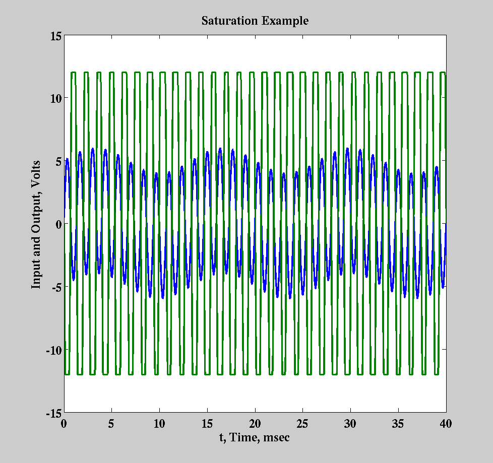
An example of saturation with two signals
t=[0:0.02:40]*1e-3;  % Time to 40 msec
f_a=750;  V_apk=5;v_A=V_apk*sin(2*pi*f_a*t);  % Signals a and b at
f_b=75;V_bpk=1.0;v_B=V_bpk*sin(2*pi*f_b*t); % two different frequencies
v_IN=v_A+v_B;                                 % Add them
v_OUT=min(max(-(R_2/R_1*v_IN),v_OUTn),v_OUTp);% Output including saturation
fig4=figure;plot(t*1000,v_IN,t*1000,v_OUT);
xlabel('t, Time, msec');
ylabel('Input and Output, Volts');
title('Saturation Example');
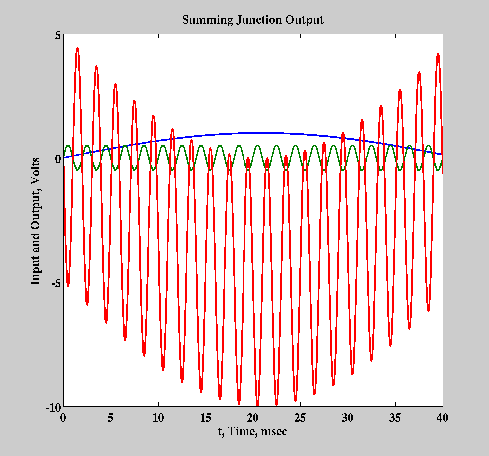
Summing Junction with two signals
R_1a=1000;R_1b=500;
f_a=12;  V_apk=1;v_A=V_apk*sin(2*pi*f_a*t);
f_b=500;V_bpk=0.5;v_B=V_bpk*sin(2*pi*f_b*t);
v_OUT=min(max(-(R_2/R_1a*v_A+R_2/R_1b*v_B),v_OUTn),v_OUTp);
fig5=figure;plot(t*1000,v_A,t*1000,v_B,t*1000,v_OUT);
xlabel('t, Time, msec');
ylabel('Input and Output, Volts');
title('Summing Junction Output');
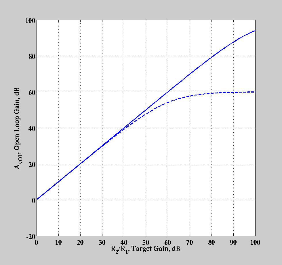
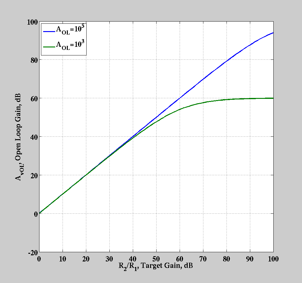
Non-Ideal Op Amps: Finite Gain
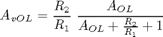
targetgaindB=[0:100];  % Our desired gain in dB
targetgain=10.^(targetgaindB/20); % R_2/R_1
A_OL=1e5;
A_vOL=-targetgain.*A_OL./(A_OL+targetgain+1);
actualgaindB=20*log10(abs(A_vOL)); % Remember the abs because voltage gain is
                                  % negative
figure;plot(targetgaindB,actualgaindB,'-');grid on;
xlabel('R_2/R_1, Target Gain, dB');
ylabel('A_{vOL}, Open Loop Gain, dB');

hold on;  % Put the next curve on the same plot
A_OL=1e3;
A_vOL=-targetgain.*A_OL./(A_OL+targetgain+1);
actualgaindB=20*log10(abs(A_vOL)); % Remember the abs because voltage gain is
                                  % negative
plot(targetgaindB,actualgaindB,'--');
hold off;

% A slightly more graceful way to do this plot;
A_OL=1e5;
A_vOL=-targetgain.*A_OL./(A_OL+targetgain+1);
actualgaindB1e5=20*log10(abs(A_vOL));  % Give the output a different name

A_OL=1e3;
A_vOL=-targetgain.*A_OL./(A_OL+targetgain+1);
actualgaindB1e3=20*log10(abs(A_vOL));
fig6=figure;plot(targetgaindB,actualgaindB1e5,...
                 targetgaindB,actualgaindB1e3);grid on;
xlabel('R_2/R_1, Target Gain, dB');
ylabel('A_{vOL}, Open Loop Gain, dB');  % Plotting both in one plot command
                                        % makes the colors different.
                                        % Why didn't that happen the first
                                        % time?
legend('A_{OL}=10^5','A_{OL}=10^3','Location','NorthWest');
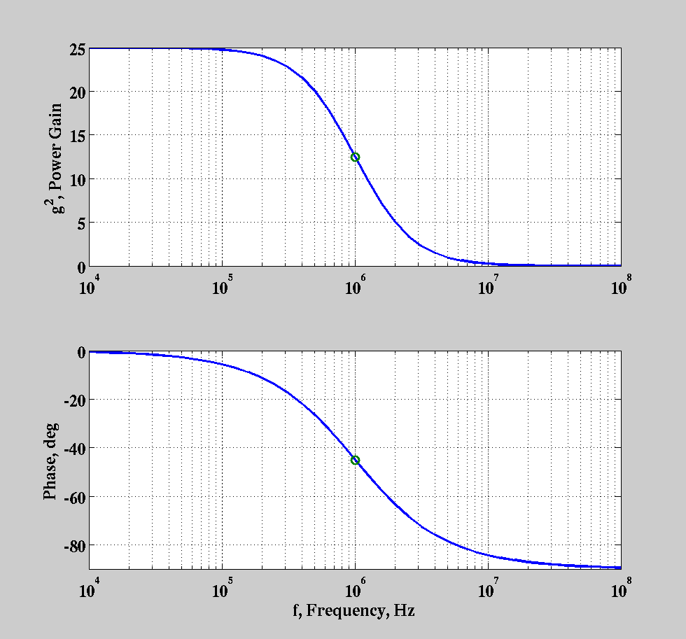
Lorentzian Spectrum to be used for gain-bandwidth analysis

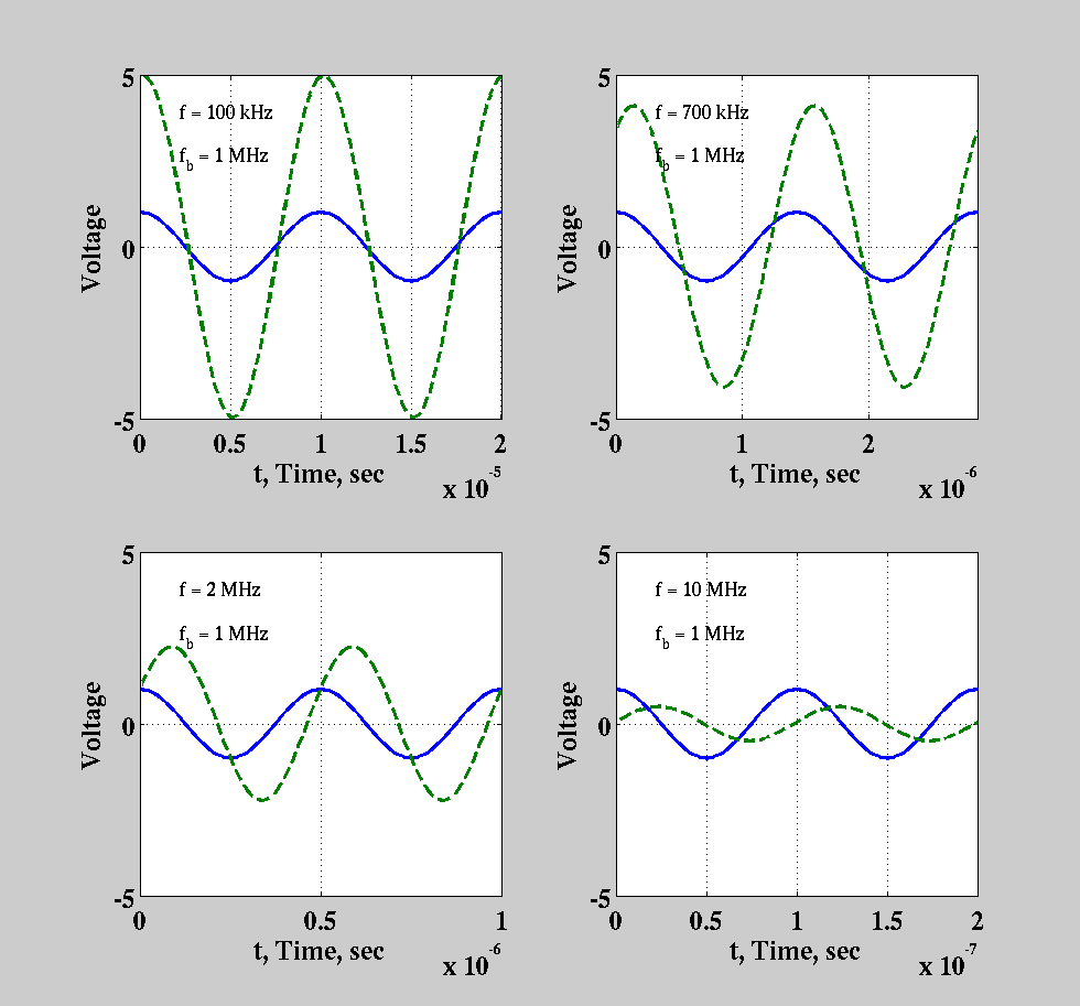
g0=5;  % Gain at zero frequency
fb=1e6;  % Bandwidth
% Plot the spectra of amplitude and phase
f=10.^[4:0.1:8];  %
g=g0./(1+j*f/fb);
fig8=figure;
subplot(2,1,1);semilogx(f,abs(g).^2,'-',fb,abs(g0)^2/2,'o');grid on;
ylabel('g^2, Power Gain');
subplot(2,1,2);semilogx(f,180/pi*angle(g),'-',fb,-45,'o');grid on;
moose=axis;axis([moose(1:2),-90,0]);
xlabel('f, Frequency, Hz');
ylabel('Phase, deg');

% Now show some examples at specific frequencies
%
%
freqlist=[1e5,7e5,2e6,1e7];% operating frequencies
fig9=figure;
for n=1:4;
  f=freqlist(n);
  g=g0/(1+j*f/fb);
  %
  % Plot time history for a couple cycles
  t=[0:0.01:1]*2/f;
  v_IN=exp(j*2*pi*f*t);
  v_OUT=v_IN*g;
  subplot(2,2,n);
  plot(t,real(v_IN),'-',t,real(v_OUT),'--');grid on;
  if f<1e6; % Write the frequency on the plot
    text(t(12),4,['f = ',sprintf('%0.0f',f/1e3),' kHz']);
  else;
    text(t(12),4,['f = ',sprintf('%0.0f',f/1e6),' MHz']);
  end;
    text(t(12),2.5,['f_b = ',sprintf('%0.0f',fb/1e6),' MHz']);
    axis([t(1),t(end),-5,5]); % Fix the axes
  xlabel('t, Time, sec');
  ylabel('Voltage');
end;
%
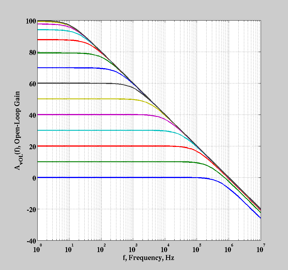
Non--Ideal Op Amp: Gain and Bandwidth
faxis=10.^[0:0.1:7];  % Frequency axis for spectrum
targetgainaxis=10.^([0:10:130]/20); % Several gains
[targetgain,f]=meshgrid(targetgainaxis,faxis);  % Make these 2-D arrays
A_0OL=1e5;
f_BOL=1e6/A_0OL
A_vOL=-targetgain./(1+(targetgain+1)./A_0OL.*(1+j*f/f_BOL));
fig7=figure;semilogx(f,20*log10(abs(A_vOL)));grid on;
xlabel('f, Frequency, Hz');
ylabel('A_{vOL}(f), Open-Loop Gain');
f_BOL =
    10