Contents

% /home/dimarzio/Documents/working/12229/lectures/rc2students.m
% Thu Oct 19 15:09:09 2017
% Revised Tue Oct 23 17:55:10 2018
% Chuck DiMarzio
tmax=1024;t=[1:tmax]; % Time in units of dt

Periodic signals

A couple of simple functions to use

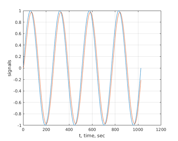
sine256=sin(2*pi*t/256); % period is 256 sec, f=(1/256) Hz
square=double(sine256>0); % Easy way to make a square wave.


a=0.1; % a = dt/(RC)

figure;measurement=rcfilter(t,square,a);
hold on;
moose=axis;
plot(moose(1:2),exp(-1)*[1,1],'k--');
plot(moose(1:2),(1-exp(-1))*[1,1],'k--');
hold off;

figure;measurement=rcfilter(t,sine256,a);

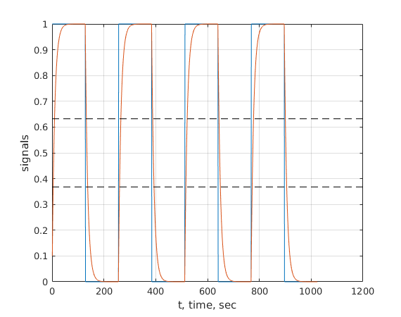
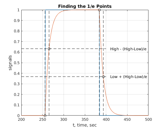
Measuring the time constant

figure;measurement=rcfilter(t,square,a);
hold on;
moose=axis;moose(1)=200;moose(2)=500;axis(moose);
plot([moose(1),400],exp(-1)*[1,1],'k--');
plot([moose(1),400],(1-exp(-1))*[1,1],'k--');
plot(256*[1,1],moose(3:4),'k--');plot(256,0,'ko');
plot(265.5*[1,1],moose(3:4),'k--');plot(265.5,1-exp(-1),'ko');
plot(384*[1,1],moose(3:4),'k--');plot(384,1,'ko');
plot(393.5044*[1,1],moose(3:4),'k--');plot(393.5044,exp(-1),'ko');
text(410,exp(-1),'Low + (High-Low)/e');
text(410,1-exp(-1),'High - (High-Low)/e');
title('Finding the 1/e Points');
hold off;

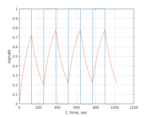
Try making a smaller and see what happens.

a=0.01; % a = dt/(RC)

figure;measurement=rcfilter(t,square,a);
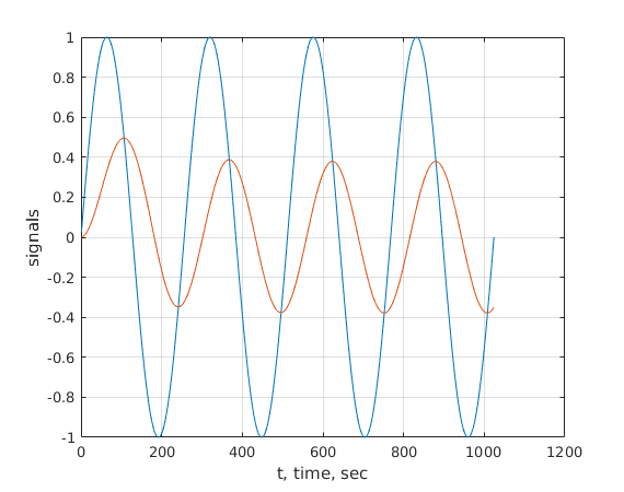
figure;measurement=rcfilter(t,sine256,a);

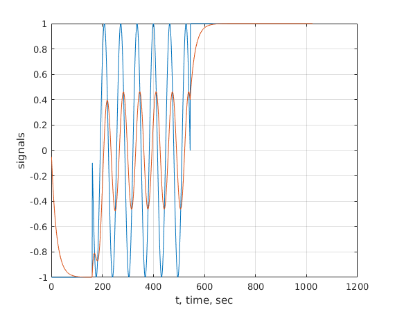
Burst periodic signal

a=0.05; % a = dt/(RC)
wsine64=sin(2*pi*t/64); % period is 64 sec, f=(1/64) Hz
wsine64([1:+128+32])=-1;
wsine64([513+32:end])=1;
figure;measurement=rcfilter(t,wsine64,a);

% -------------------------------------------------------------------

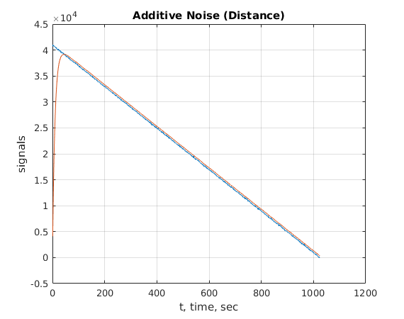
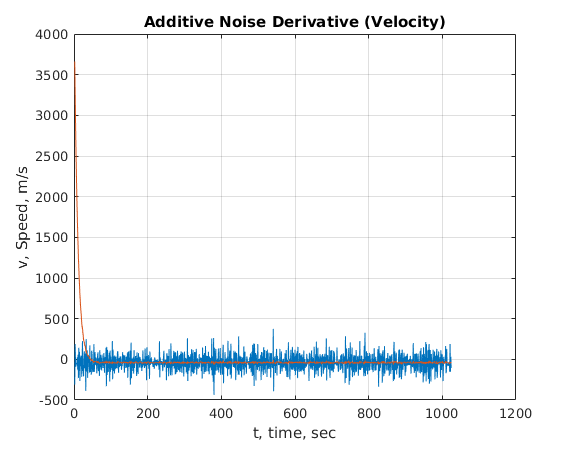
Radar signal

%  I will explain the radar signal in class.  In this case, the
%  object is coming toward the radar, arriving (distance=0) at time
%  tmax.

a=0.1; % a = dt/(RC)

speed=40;noisedist=80; % Simulated police radar signals; 40 meters
                       % per second is kind of fast.
distance1=speed*(max(t)-t); % Ideal signal
distance2=distance1+noisedist*randn(size(t)); % Noisy signal
ttest=double(rand(size(t))>0.99);  % Noisy signal with dropouts
distance3=distance2.*(1-ttest)+tmax*speed*rand(size(t)).*ttest;

% Plot the noisy distance measurement and filtered one.
figure;measurement=rcfilter(t,distance2,a);
title('Additive Noise (Distance)');

% Range rate is distance difference divided by time difference
figure;plot(t(2:end),distance2(2:end)-distance2(1:end-1),...
     t(2:end),measurement(2:end)-measurement(1:end-1));grid on;
xlabel('t, time, sec');ylabel('v, Speed, m/s');
title('Additive Noise Derivative (Velocity)');

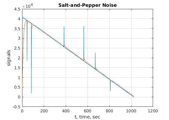
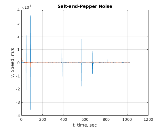
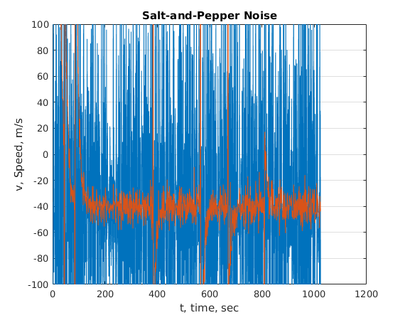
Salt and Pepper Noise (linear filters don't work very well)

figure;measurement=rcfilter(t,distance3,a);
title('Salt-and-Pepper Noise');
figure;plot(t(2:end),distance3(2:end)-distance3(1:end-1),...
     t(2:end),measurement(2:end)-measurement(1:end-1));grid on;
xlabel('t, time, sec');ylabel('v, Speed, m/s');
title('Salt-and-Pepper Noise');

% Fix the speed scale to show reasonable values
figure;plot(t(2:end),distance3(2:end)-distance3(1:end-1),...
     t(2:end),measurement(2:end)-measurement(1:end-1));grid on;
xlabel('t, time, sec');ylabel('v, Speed, m/s');
moose=axis;axis([moose(1:2),-100,100]);
title('Salt-and-Pepper Noise');

% Try different filters (ie. change a).  A long time constant
% provides a smoother distance curve which gives better velocity
% measurements, but will take longer to respond to changes in
% speed.

Published with MATLAB® R2017a